Permeability Estimation From Inflow Data During Underbalanced Drilling
Unlocking Reservoir Insights: Permeability Estimation from Inflow Performance Relationship (IPR)
 |
| Permeability Estimation From Inflow Data During Underbalanced Drilling |
Abstract
Underbalanced drilling has become increasingly popular as it reduces formation damage caused by fluid invasion during drilling operations. This is particularly important in the case of depleted reservoirs or when horizontal and deviated wells are drilled with long exposure time. As a result of the lower pressure in the wellbore, there is an inflow from the reservoir into the wellbore, which is continuously measured at the wellhead. This inflow carries information about the reservoir. The objective of this paper is to develop a mathematical model and its associated interpretation methods to estimate reservoir permeability and its variation along the length of a horizontal wellbore using the inflow measurements at the wellhead.
The traditional methods of pressure and rate transient analysis are not applicable to underbalanced drilling data, particularly because the length of the producing interval is continuously increasing with time. In this paper, we will develop a mathematical model accounting for this complication. This model calculates inflow rates in the forward mode and the reservoir permeability when used in the backward mode.
We have validated our methodology against synthetic data obtained from numerical simulation, and applied it to a number of actual field cases. In field studies, after estimation of the permeability profile along the wellbore, the estimated permeabilityvalues were used along with reported bottomhole pressure rightafter the end of drilling to calculate gas inflow. This was then compared with the measured total inflow. Good agreement was obtained between the predicted and measured values. In another field case, we successfully predicted the long-term gas production of the well. In addition, our calculated average permeability value was comparable to the one obtained from a well test analysis performed later in the life of the well. Furthermore, a series of studies were conducted to examine the sensitivity of the estimated permeability to errors in the reported inflow information and the pressure drop along the wellbore. The results reported in the paper indicate that the estimated permeability profile remained relatively unchanged.
Introduction
Formation testing during underbalanced drilling (UBD) relies on the hypothesis that the inflow rate contains enough information from the reservoir to enable the determination of some reservoir
properties. Acquisition of the flow rate and bottomhole pressure data, and their analysis, can offer information about the permeability and its variation along the length of the wellbore.
A nalyzing the UBD data has been the subject of many papers; some of the more recent ones are reviewed below.
Hunt and Rester(1) modified the standard pressure transient analysis techniques to include time-dependent boundary conditions, which account for the variable well length as the drilling bit progresses in the reservoir. The reservoir parameters are calculated based on a trial and error procedure as part of a history-matching exercise. A more recent paper by the authors(2) extends this to multilayer reservoirs.
Kneissl(3) suggests introducing fluctuations to the bottomhole pressure during drilling to calculate both the permeability and the pore pressure during UBD. Similarly, Vefring et al.(4) show that introducing fluctuations to bottomhole pressure while drilling can improve the estimation results for simultaneous calculations of permeability and pore pressure. In this paper by Vefring et. al.(4), as
well as in earlier work by the authors(5), they tie in a dynamic well flow model with a simple transient reservoir model.
Biswas et al.(6) focus on estimating the reservoir permeability, employing a two-phase, 2D transient reservoir simulator coupled with a transient multiphase wellbore model. The optimization for
calculating permeability is done with a genetic search scheme. The pore pressure is assumed to be known, and the problem of nonunique solutions has also been addressed.
The objective of this paper is to develop a simple method for the determination of permeability along the length of a horizontal wellbore.
The data that we worked with exhibits large fluctuations in recorded wellbore rates. This is because the operator continuously adjusts the gas injection rate and the back-pressure to achieve a desired underbalance. Such adjustments could be quite frequent, which, when combined with the well passing through a reservoir of varying permeability, can lead to significant changes in the inflow
rate. In this paper, we will not focus on interpretation of each spike in recorded flow rate; instead, we will develop a methodology that allows quantification of a number (e.g. a handful) of permeability features along the length of a wellbore. An average permeability is then obtained, which may be used for forecasting flow rate with time. Two field cases are used to demonstrate the applicability of this methodology. Furthermore, the results of this work may be used to examine the presence of an areal permeability pattern among a number of wells drilled in a particular area of a reservoir. This information could then be compared with independent evaluations of areal permeability variations with the use of geological and geophysical information. Such information is then used for decisions about well placement, etc. This paper focuses on the development, validation and field application of a methodology for determination of permeability along the length of a horizontal wellbore during underbalanced drilling.
The problem statement, methodology and mathematical model are presented next. This is followed by validation against synthetic data and the analysis of two field cases. The possibility of obtaining other interpretations (non-uniqueness) is then addressed through a set of sensitivity studies, before the discussion and the conclusion are given.
Problem Statement
The objective of this work is to identify and quantify high and low permeability zones along the horizontal well by processing the inflow data during UBD.
As drilling progresses, the wellbore length increases and the measured flow rate changes in response to increased length and the changing conditions (e.g. bottomhole pressure and drilling rate).
These complications require modification of conventional analysis techniques used in well test analysis.
To account for the changing length of the wellbore during drilling, we divide the wellbore into a number of sections, which we name segments. We seek the determination of permeability for
each segment. The permeability and drilling rate are assumed constant for each segment, as well as the bottomhole pressure during the drilling of each individual segment. Based on the solution of
the diffusivity equation to appropriate boundary conditions, we have developed a model to calculate the flow rate in a constant permeability section of a horizontal well (i.e. a segment) at a known
bottomhole pressure. This model, which requires the knowledge of permeability, and results in the calculation of the inflow rate, is called the “forward” model. It accounts for the production into the
segment while drilling (changing length), and also calculates inflow into that fixed length segment after the drilling is completed.
When the inflow rate into a fixed-length segment is known, the same model is used in “backward” mode to calculate the permeability of that segment. As explained in the following, to obtain the
permeability profile, we employ the backward and forward models alternately.
The measured inflow data during the drilling of the first segment is analyzed along with the measured bottomhole pressure to obtain permeability of that segment employing the backward model. To
calculate the permeability of the second segment, we require the gas influx from the second segment. However, the measured rate includes the rate from the first and second segments. To correct
for this, the gas produced by the first segment during the drilling of the second segment is calculated and subtracted from the measured wellbore influx during this time. This yields the gas inflow
for the second segment alone. The latter is used in the backward model to calculate its permeability. This process is continued until the wellbore is drilled fully, and the permeability profile is calculated.
Once the drilling is complete, the forward model is used to forecast the gas production rate from all segments and this is compared with measured rate vs. time.
Through experience, we learned that we need to compliment the above approach with a second approach, which is strictly based on the use of the forward model. We found that, at times, and as
a result of big spikes in the input data, the measured inflow may become less than the calculated inflow from the preceding segments.
To avoid this, we choose the permeability of each segment such that it matches the corresponding inflow (forward modelling) while allowing for the calculation of a positive permeability for
the subsequent sections. Fekete has developed a software application which allows importing, filtering and analysis of the data using both approaches and reports the permeability profile along
the length of the wellbore, as well as the gas production rate with time.
Methodology
We consider a segment of a horizontal wellbore that is being drilled in a reservoir, bounded with no-flow boundaries at the top and bottom, and we develop a solution for the cumulative gas production
while that segment is being drilled (see Figure 1). We choose an analysis based on cumulative gas production (during the drilling of each segment) because it will be less affected by the noise in the data. Furthermore, we choose the segments such that the time of drilling of each segment is larger than the time scale of transient effects within the wellbore. This minimizes the errors in the determination of reservoir influx rates. The influx rate from the formation is calculated by subtracting the injected gas rate (to maintain a low density fluid in the wellbore) from the total gas outflow rate from the wellbore. The following is a list of other assumptions used and the implications of each:
1. The reservoir is horizontal, heterogeneous and isotropic. The reservoir has a constant thickness, h, a constant porosity, φ, and an infinite lateral extension (production during drilling does not cause reservoir depletion).
2. The radial flow in the vertical plane is ignored. The pressure drop due to convergence of the flow lines approaching the wellbore is accounted for by a geometric skin,
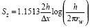
where h is the reservoir thickness, rw is the wellbore radius and Δx is the length of the segment(7). It has been shown(7) that this is a good approximation when the dimensionless time based on reservoir thickness is larger than 0.15. Using this criterion, it can be shown that the approximation caused
by this assumption is acceptable for a reservoir of small thickness, particularly in segments with higher permeability.
For a reservoir studied in this paper (i.e. thickness of about 6 m) it is found that the linear flow with geometric skin is a good approximation when permeability is more than 0.05 mD. When permeability is significantly less, our calculated permeability is optimistic. This approximation did not cause any limitation in this study, since the reservoir section with a permeability less than 0.05 mD did not contribute much to the overall flow. For other cases, when representation of radial flow using a steady-state skin term is insufficient, incorporation of more complete solutions that account for early
radial flow and late-time linear flow is possible.
3. Flow is 1D perpendicular to the wellbore (i.e. flow inside the reservoir, parallel to the wellbore, as well as vertical flow, are ignored). Yu(8) showed that this approximation is valid when the rate of penetration, u, is large as compared with the rate of pressure propagation along the wellbore, η/L. A dimensionless group was defined as Pe = uL/η, and it was found that 2D flow in the reservoir (and parallel to the wellbore) may be ignored when Pe > 10. For the cases studied here, it was found that the 1D approximation is valid when permeability is less than about 100 mD. This is generally the case with the reservoir of interest in this paper, except if fractures are intersected. In such a case, pressure would decline very quickly in the fracture, leading to cross-flow from the matrix into the fracture. For the case of small fractures (with limited connectivity to other fractures), we expect spike-like gas rates and fast depletion of the fracture. This motivated the idea of segmenting the wellbore into longer segments to compensate for the short, high permeability section which will deplete fast. In case of a long fracture (connected to other fractures), we observe its effect as a long duration of high influx, and analyze accordingly. Nevertheless, in the presence of a fracture, contribution of flow from adjoining rocks initiates a 2D flow (depending on the length of the fracture). In this work, the effect of a fracture is represented by the calculation of an increased permeability of the segment where the fracture is located.
4. Bottomhole pressure is assumed constant along the wellbore, however, bottomhole pressure may vary as new segments are being drilled. Furthermore, the effect of pressure drop along the wellbore has been analyzed in the Sensitivity Studies section and found to be insignificant.
5. Mechanical skin of zero is assumed. This is thought to be reasonable for the case of underbalanced drilling conditions.
Should there be a mechanical skin, this analysis will provide a measure of the productivity (as opposed to permeability) and its variation along the wellbore.
The validity of some of these assumptions is examined under the sections entitled Sensitivity Studies and Discussion, below.
Mathematical Model
Consider a semi-infinite reservoir representing half of the reservoir, which is infinite only in one direction, perpendicular to the wellbore (y direction). The flow from the infinite reservoir (fulldomain) will be twice this flow, assuming no interference between the two sides.
Using the assumptions stated previously, the 1D diffusivity equation may be used to describe the instantaneous single-phase flow of gas towards a well of length Δx as:
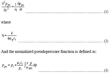
Although the term μgct is a function of pressure, we can assume it is constant, because the average reservoir pressure during the short time of drilling does not change. This has been shown to be a good approximation in many references(9, 10). Here we represent the boundary conditions while the well is drilling. For the period of time after the well has stopped drilling, the value of x will be constant (no longer increasing with time).
Initial condition:


where Δx is the length of the particular segment and Δt is the time it took to drill it.
The full-domain (flow from both sides) analytical solution of the above problem is presented in two parts. The first, Equation (9), gives the influx during the continuous drilling of a segment, and the second, Equation (12), gives the influx after the segment has been drilled. As stated previously, the use of cumulative production (instead of instantaneous rate) is advantageous, because it allows working with very noisy rate data. While drilling, the cumulative flow for a particular segment is given by:

For a segment that is being drilled, the permeability is calculated using the backward model [Equation (9)] given a flowing pressure and a quantity of produced gas. Since this equation is a nonlinear function of permeability, k, we incorporate an iterative algorithm to solve for k. For the first drilled segment, the quantity of produced gas during the drilling of that segment is known a priori by actual measurement of the flow rate. For subsequent segments, this value is not known directly, and must be determined as described below.

While a subsequent segment is being drilled, the measured production, Q(meas) consists of two components: (i) the new influx Q(new) from the segment currently being drilled, and (ii) the continuing flow Q(old) from the previously drilled segments. Because the permeability values of the previously drilled segments have already been determined, the continuing flow contribution Q(old)
from those segments can be determined using the forward model [Equation (12)]. The influx from the new segment being drilled can now be calculated by simply subtracting Q(old) from Q(meas).
In the situation where the bottomhole pressure changes with time, the gas production in the forward model [Equation (12)] is calculated using superposition in time.
Validation Against Simulation Data In this section, we assess the accuracy of our methodology by
analyzing simulated drilling data. A commercial reservoir simulator (CMG 2000) was employed to generate underbalanced drilling data. The total well influx is then analyzed with our methodology
described above, and the resulting permeability profile is compared with the permeability values used as inputs into the simulator.
The simulator models a horizontal well of radius, rw, being drilled in the x direction in the middle of a finite, heterogeneous
isotropic gas reservoir. The reservoir is limited to impermeable boundaries in the vertical z direction. Furthermore, the boundaries in the y direction are chosen far enough so that the effect of depletion during drilling is not felt at those boundaries. Known and constant initial reservoir pressure is considered (see Table 1).

Table 1 gives the parameters used for the simulation. The case represents a heterogeneous reservoir that is being drilled at a rate of 20 m/hr at a constant bottomhole pressure.
Figure 2 shows the simulated inflow data along with the rate of drilling and bottomhole pressure. The data of Figure 2 were used as input data and analyzed based on the methodology described earlier. Figure 3 shows the estimated permeability, as well as the values used in the simulator. A close agreement is seen between the input permeability values and the ones calculated using our approach.
Field Results
In this section, two sets of field data are analyzed to determine formation permeability.
The first set of data belongs to a 1,200 m horizontal wellbore.
The data has two parts. The first part is while the well is being drilled, consisting of the bottomhole pressure, drilling rate and the inflow rate. This data is used to calculate the permeability profile.
The second part is after the drilling has stopped. The data consists of inflow rate and flowing pressure for a few hours after the drilling has finished. We predict the gas inflow using the estimated
permeability profile. We compare this calculated flow rate to the measured gas rate after drilling.
 Figure 4 shows the algorithm used in the software for calculating the permeability of the nth segment along the wellbore. After segmenting the wellbore into smaller sections, the pressure values
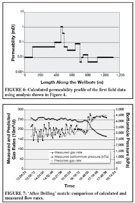
measured during the drilling of every segment are averaged, and the corresponding cumulative production is calculated. The data of the first segment is used in the backward model to calculate its permeability.
The difference between cumulative production during drilling of the new segment and that from previous segments (calculated using the forward model) is fed into the backward model, yielding the permeability of the new segment.
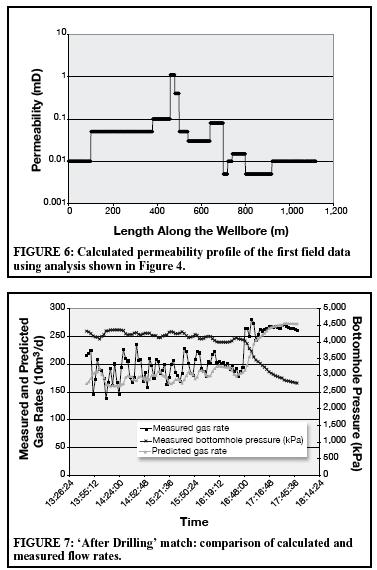
The results are shown in Figures 5 and 6. Figure 5 shows the comparison between measured and calculated inflow during drilling and Figure 6 presents the permeability profile of the formation versus length. The results shown in Figures 5 and 6 indicate that the first 80 m of the wellbore has a permeability of around 0.01 mD, followed by 750 m of 0.05 to 0.1 mD permeability formation,
with a notable exception of a high permeability region at around 500 m. The last third of the well exhibits a permeability of around 0.01. This analysis suggests that the majority of production in this
wellbore will be from its middle region.
After the end of drilling, the measured bottomhole pressure and the previously calculated permeability profile (Figure 6) were used to predict the inflow rate after drilling. The results shown in Figure 7 demonstrate a close agreement between the measured and predicted inflow rates.
The second set of field data has been recorded while drilling a 1,000 m horizontal well (Figure 8). Drilling was suspended for about a day. While there is not a depth available for this period, the
operator maintains that the well remained underbalanced. We employ this drilling data to calculate the permeability profile. Three permeability regions are observed in Figure 9. The first and last regions are of higher permeability, whereas the middle region has a lower permeability profile.
The calculated permeability profile has then been employed to forecast the long-term production of this well. Figure 10 presents a comparison of the forecast results and the measured gas rates over
the first year of production. Very good agreement is observed between the two sets of data

The next step is to compare the results of our analysis with those obtained from a conventional well test analysis. This well test analysis has been done later on in the life of the well. For such a comparison, we require an approach to obtain an average permeabilityvalue from the permeability profile.
Average Permeability
The permeability along the wellbore varies significantly. We have considered different methods of averaging. The flow regime used in the analysis is transient linear flow, and the mathematics of linear flow analysis does not yield permeability, but rather the product Δx√k. We demonstrate later on in this paper that the sum (ΣΔx√k) is insensitive to segment length and we note (not shown here) that a simple arithmetic averaging of permeability, using the summation ΣΔx × k, rather than ΣΔx√k, does not give consistent results for the various segment lengths. Accordingly, we maintain that an average permeability along the wellbore is best obtained from (ΣΔx√k)/ΣΔx.

Figure 11 demonstrates cumulative transient productivity as the well is being drilled. Average permeability for a fully drilled well has been calculated as kav = 0.017 mD, which is in close agreement with the results of the independent well test analysis where kH = 0.03 mD and kV = 0.02 mD.
Sensitivity Studies
Many factors can potentially affect the results of our analysis. In this section, we evaluate the sensitivity of our results to three parameters. The factors that we investigate and a description of
the analyses are given in three parts. Part 1 will investigate the effect of measurement error, Part 2 will look at the effect of pressure drop along the wellbore and Part 3 will examine the effect of segment size.
Part 1: Presence of Measurement Error and Noise in Production Data
To investigate the sensitivity of results to the presence of measurement error, random noise with a standard deviation of 10% is added to the reported gas rate. A constant segment length of 20 m is used. The results (not shown here) demonstrate that the evaluated permeability profile is not significantly altered by the addition of error. This is because the permeability values span 3 to 5 orders of magnitude in logarithmic scale. Changes of the order of 10% in production data affect the resulting permeability values to the same extent, and have little effect on the overall permeability profile.
Part 2: Pressure Drop Along the Length of the Wellbore
The pressure gauge, which is located a couple of 10’s of metres behind the drilling bit, provides the downhole pressures used in this study. It was expected that the pressure drop along the length of the
wellbore is small and, therefore, will not affect the interpretation of the results. However, it had been suggested that if pressure drop along the wellbore has a significant effect on the estimated permeability profile, it may be necessary to install a second downhole gauge at some distance away from the first one, and measure the actual pressure drop. We have evaluated the effect of pressure
drop along the horizontal wellbore on the permeability profile by accounting for a pressure drop of 0.1 kPa/m with a constant segment size of 20 m. The results (not shown here) indicated that the permeability profile is not affected by such pressure drops. Therefore, an actual measurement of pressure drop along the wellbore is not necessary unless the bottomhole pressure is much closer to the reservoir pressure.
Part 3: Segment Length
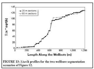
The actual well is continuous and not segmented. Segmenting is something that we have introduced to allow the interpretation that permeability is assumed constant along every segment. In this section, we examine the sensitivity of the results to the length and number of segments. The use of small segments usually results in large jumps in the estimated permeability profile. Very long segments, on the other hand, can mean loss of information along the wellbore. Ultimately, it is the experience of the analyst that determines the selection of the segments. However, to evaluate the effect of segmenting on the permeability profile, two different segmentation cases are considered. Note that this is not the same well as that of Figures 5 to 11. Two different segment lengths are considered:
20 m segments and 60 m segments. The results, shown in Figure 12, indicate that while using segments of smaller size results in more fluctuations in the estimated permeability values, the
overall signature of permeability profile remains unchanged. For example, regardless of the segment size used, the results indicate that the second quarter of this wellbore length has the highest permeability values, while the first quarter has almost no permeability.
The third and fourth quarters of the wellbore have permeability of the order of 0.01 mD or lower. Figure 13 shows a measure of the cumulative transient productivity, ΣΔx√k, for the three interpretations.
Close agreement between the two cases is observed. This is also confirmed when the predicted gas flow rate after drilling is completed showed no dependence on the segment size chosen, and demonstrated a close agreement with the measured flow rate.
The sensitivity studies shown here suggest that the estimated permeability profiles are not affected by some of the errors and causes of uncertainty.
Discussion
In this section, we would like to answer the following two questions:
1) do errors in permeability estimation in this work accumulate; and,
2) how unique is the obtained permeability profile?
We will also discuss the possibility of obtaining ‘negative’ permeability, and how we have dealt with it.
1. Do Errors in Permeability Estimation Accumulate?
The short answer is no. This answer can be explained using the following example. Assume a homogeneous reservoir with a permeability of 10 mD that has been divided into three segments for
analysis. Assume that somehow the permeability of the first segment is estimated to be 15 mD. The permeability of the second segment is calculated by subtracting the contribution of the first
segment from the total measured influx. With an overestimated permeability for the first segment, the contribution of the first segment would be overpredicted, resulting in an underprediction of
contribution of the second segment, which, in turn, results in a permeability value less than 10 mD. By the time the permeability of the third segment is to be evaluated, we will have an overestimation
in contribution of the first segment and an underestimation in contribution of the second segment. These effects compensate for each other (at least partially). While we have not investigated
whether these errors totally cancel each other or not, this example shows that they do not compound each other.
2. How Unique is the Estimated Permeability Profile?
Unfortunately, the answer to this question is not as simple as the first one. While a number of sensitivity studies conducted in this study showed that the resulting permeability profiles remained
relatively unchanged, we have not fully explored conditions that could result in non-unique permeability fields. Nevertheless, we have observed significant differences in the estimated permeability values under the following scenarios:
i) When a low permeability section appears after a high permeability section, resulting in some error in estimation of the high permeability value. This is because when a low permeability
zone appears after a high permeability zone, the contribution to inflow of the low permeability zone is very small.
An error in estimation of the preceding high permeability zone will result in significant error in estimation of the contribution of the new segment, resulting in significant error in estimation of the permeability of the low permeability segment.
This can result in non-uniqueness in estimation of permeability of the low permeability segments that appear after high permeability segments. In fact, we have frequently faced scenarios where, after calculation of a high permeability value for a segment, the calculated contribution for the next segment has become negative! This may be due to depletion of fractures that have exhibited a high permeability behaviour, but have not been able to continue to contribute as expected because they have quickly depleted. This situation can also happen because of some error in estimation of the high permeability value. When we have been faced with this situation of negative contribution for the new segments, we have tried changing the segment size and/or adjusting the permeability of the high permeability zone. In some cases, however, when this was not warranted, we have chosen a value of 0.0001 mD for the new segment.
ii) Another case that could cause some form of non-uniqueness in results, is when the size of segments was reduced significantly.
In such cases, we would observe significant fluctuation in the permeability field, which we anticipate to be (at least partially) because of the fluctuating inflow data. As it was shown earlier, the overall transient productivity of the wellbore remains independent of segmenting.
Summary and Conclusions
We have developed an analytical model for the estimation of permeability along the length of a horizontal wellbore that is drilled underbalanced. The permeability values of these segments are estimated as they are being drilled, through a combination of forward and backward modelling. The methodology accounts for variable bottomhole pressure and a variable rate of drilling. The model was validated using synthetic data and was used to analyze several sets of field data. Based on the results of these studies, the following conclusions are made:
• The estimated permeability profile was successful in predicting the production rate after the completion of drilling.
• A number of sensitivity studies indicated that the permeability field was relatively unique. In particular, the overall transient productivity of the wellbore remains unchanged.
• Averaging the well’s permeability should be done on the basis of √k.


Comments